Removing Dupes in Excel with Formulas

A clean and well-structured dataset is every data analyst's dream. However, we don’t get perfect datasets in a world full of imperfections. We make one. And how? Excel.

So, in this blog post, we’ll learn how to remove duplicates in Excel with Formula.

Step 1:

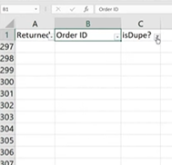
In the data set where you want to remove duplicates, add an “isDupe?” column. The column will act like a little visual indicator.

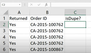
Step 2:

In the cell below the “isDupe?” header, type formula that counts how many times a particular value appears in the dataset below.

=COUNTIF(B3:$B$801,B2)

The formula checks the numbers below the number we want to see if the dupes exist, implying that we want to count if a selected value appears in the remainder of the dataset.

The dollar sign fixes the end value, i.e., no matter where we copy this formula down, the reference will be absolute, meaning it always ends at that specific cell.

Upon hitting Enter, we get 3 in cell C2 for this particular dataset, which means CA-2015-100762 appears three times below cell B2 in the entire selected range.

Step 3:

Double click on the bottom right corner of cell C2 to copy this formula down the column.

Notice as we move down the column, B801 doesn't change while the rest of the formula does because of the absolute reference.

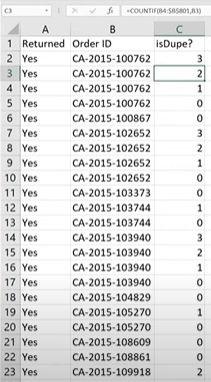
Now what we have is a column that identifies when we have dupes. Anything above zero means there is a duplicate in the dataset.

To make it a little bit easier to read, let’s put an if statement around it.

Step 4:

Edit the COUNTIF formula to make it a conditional IF statement using the following formula and press Enter

=IF(COUNTIF(B3:$B$801,B2)>0,1,0)

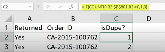
The interpretation of the formula is, “If the count of selected number (B2) is greater than 0 in the range below that number (B3 to B801), then the output should be “1” (True) else “0” (False).”

Instead of showing a 3 in cell C2, we see 1, i.e., “True.”

Step 5:

Double click on the bottom right corner of cell C2 to copy the formula down the column.

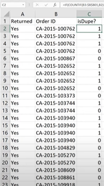
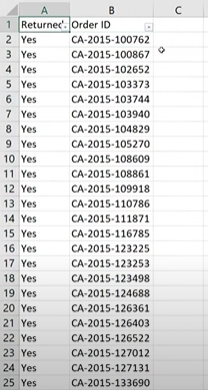
Now we have only 0s and 1s in “isDupe?” column. We can simply use a filter and delete all the rows where “isDupe?” is 1 (True aka duplicate)

Step 6:

Click over on Sort and Filter, uncheck the zero. Select all the rows where “isDupe?” is 1, right click, and select Delete row.

Now, go back to filter. Clear it (you can see we don't have any more ones here). In fact, the bottom-most row shows an error because it's trying to count something that doesn't exist anymore.

Step 8:

Select and delete the “isDupe?” column as we no longer need that visual indicator.

Finally, we have our de-duplicated dataset that is much cleaner and easy to work with.

To learn more on all things data, head over to FreeTheDataAcademy.com/yt to see our entire catalog and sign up for a seven-day free trial so you can start learning today to elevate your career tomorrow.